Tutorial: Color Correction Pipeline
The color correction module has been developed as a method of normalizing image-based data sets for more accurate image analysis.
PlantCV is composed of modular functions that can be arranged (or rearranged) and adjusted quickly and easily. Pipelines do not need to be linear (and often are not). Please see the pipeline examples below for more details. Some functions have a optional debug mode that prints out the resulting image. The debug has two modes, either 'plot' or print.' If the global object, plantcv.params.debug is set to 'print' then the function prints the image to a file. If using a jupyter notebook, you would set debug to 'plot' to have the images plot images to the screen. Debug mode allows users to visualize and optimize steps on individual test images and small test sets before pipelines are deployed over whole data-sets.
For simple input and output, a helper function called plantcv.transform.correct_color was developed. See more information here
Important Note: This function has been developed with only 8 bit images in mind. Images of other bit depth are not compatible with this function.
Conditions
To run color correction on an image, the following are needed:
-
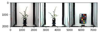
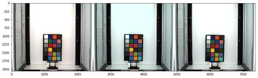
Target and source images must contain a reference from which color values are sampled. The following example uses a 24-color Colorchecker passport.
-
A target image (RGB) must be chosen. This image will be of the color profile to which other images will be corrected.
-
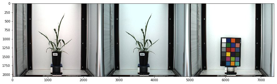
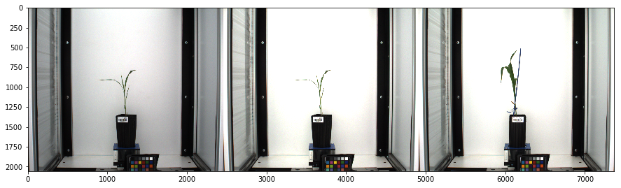
A source image (RGB), that will be corrected to the target image's color profile.
-
A mask (gray-scale) of the target image in which background has value 0, and color chips from the colorchecker are labeled with unique values greater than zero, but less than 255.
-
A mask (gray-scale) of the source image labeled consistently with the target image's mask.
To see an example of how to create a gray-scale mask of color chips see here.
Developing a pipeline
The modularity of PlantCV allows for flexible development of pipelines to fit the context and needs of users. The development of a pipeline for color correction is no different. Below are two potential scenarios with possible color correction pipelines.
Scenario A: One Target profile, One Source profile
For situations where only one source profile is identified per target profile, or one source profile will serve as a representation for many images, a simple pipeline can be developed to produce a transformation matrix that can be applied to the set of images congruent to the source profile.
1) Read in target, source, and mask images.
from plantcv import plantcv as pcv
import cv2
import numpy as np

target_img = cv2.imread("target_img.png")
source_img = cv2.imread("source1_img.png")
mask = cv2.imread("test_mask.png", -1) # mask must be read in "as-is" include -1
#Since target_img and source_img have the same zoom and colorchecker position, the same mask can be used for both.
2) Declare an output directory to which your target, source, and transformation matrices will be saved.
#.npz files containing target_matrix, source_matrix, and transformation_matrix will be saved to the output_directory file path

output_directory = "./test1"
3) Run the images through the plantcv.transform.correct_color function.
target_matrix, source_matrix, transformation_matrix, corrected_img = pcv.transform.correct_color(target_img, mask, source_img, mask, output_directory)
If you are in debug mode "plot," an horizontally stacked comparison of the source, corrected, and target images will be displayed.
4) Using either the returned transformation_matrix or loading the transformation_matrix from its directory, you may now apply the matrix to congruent images.
transformation_matrix = pcv.transform.load_matrix("./test1/transformation_matrix.npz") #load in transformation_matrix

new_source = cv2.imread("VIS_SV_0_z1_h1_g0_e65_v500_376217_0.png") #read in new image for transformation

corrected_img = pcv.transform.apply_transformation_matrix(source_img= new_source, target_img= target_img, transformation_matrix= transformation_matrix) #apply transformation
Important Note: The color correction submodule has been made with the capability to handle incomplete colorchecker data in the source image. This way if color chips have been cut off, the module will still work. Color chips do need to be consistently labeled from target to source. See an example of this here.
Scenario B: One Target profile, Many Source profiles
For situations where each source image contains a colorchecker, a pipeline may be optimized by using functions from the transform submodule. The target_matrix may be saved separately and referred to as needed for each source.
1) Read in target, source, and mask images.
target_img = cv2.imread("target_img.png")
source_img = cv2.imread("source_img.png")
mask = cv2.imread("mask.png", -1) # mask must be read in "as-is" include -1
#Since target_img and source_img have the same zoom and colorchecker position, the same mask can be used for both.
2) Save the target color matrix.
# get color matrix of target and save
target_headers, target_matrix = pcv.transform.get_color_matrix(target_img, mask)
pcv.transform.save_matrix(target_matrix, "target.npz")
3) Compute the source color matrix.
#get color_matrix of source
source_headers, source_matrix = pcv.transform.get_color_matrix(source_img, mask)
4) Get the Moore-Penrose Inverse Matrix.
# matrix_a is a matrix of average rgb values for each color ship in source_img, matrix_m is a moore-penrose inverse matrix,
# matrix_b is a matrix of average rgb values for each color ship in source_img

matrix_a, matrix_m, matrix_b = pcv.transform.get_matrix_m(target_matrix= target_matrix, source_matrix= source_matrix)
5) Calculate the transformation matrix.
# deviance is the measure of how greatly the source image deviates from the target image's color space.
# Two images of the same color space should have a deviance of ~0.
# transformation_matrix is a 9x9 matrix of transformation coefficients

deviance, transformation_matrix = pcv.transform.calc_transformation_matrix(matrix_m, matrix_b)
6) Apply the transformation matrix.
corrected_img = pcv.transform.apply_transformation_matrix(source_img= source_img, target_img= target_img, transformation_matrix= transformation_matrix)
If you are in debug mode "plot," an horizontally stacked comparison of the source, corrected, and target images will be displayed.
To deploy a pipeline over a full image set please see tutorial on Pipeline Parallelization here.
Creating Masks
"""

This program illustrates how to create a gray-scale mask for use with plantcv.transform.correct_color.

"""

%matplotlib notebook
# Use matplotlib notebook for its added features of coordinate display and zoom
from plantcv import plantcv as pcv
import cv2
import numpy as np
from matplotlib import pyplot as plt

pcv.params.debug = "plot"
img = cv2.imread("target_img.png") #read in img
pcv.plot_image(img)
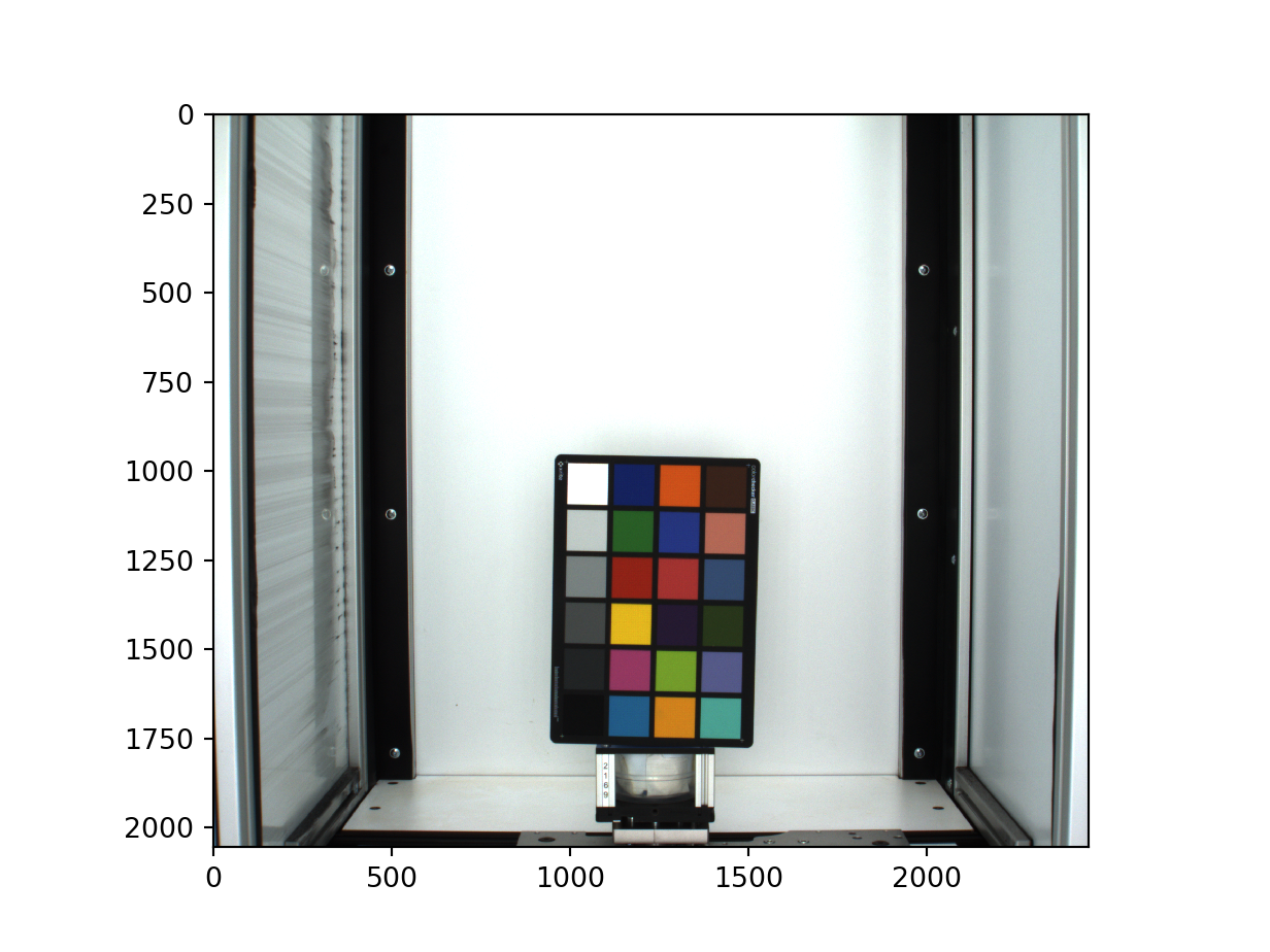
#Using the pixel coordinate on the plotted image, designate a region of interest for a 50x50 pixel region in each color chip.
#exclude white and black chips
color_1, _ = pcv.roi.rectangle(img=img, x= 1150 , y= 1010 , w= 50 , h=50 ) #blue
color_2, _ = pcv.roi.rectangle(img=img, x= 1280 , y= 1010 , w= 50 , h=50 ) #orange
color_3, _ = pcv.roi.rectangle(img=img, x= 1420 , y= 1010 , w= 50 , h=50 ) #brown

color_4, _ = pcv.roi.rectangle(img=img, x= 1020 , y= 1130 , w= 50 , h=50 ) #pale grey
color_5, _ = pcv.roi.rectangle(img=img, x= 1150 , y= 1130 , w= 50 , h=50 ) #green
color_6, _ = pcv.roi.rectangle(img=img, x= 1280 , y= 1130 , w= 50 , h=50 ) #blue
color_7, _ = pcv.roi.rectangle(img=img, x= 1420 , y= 1130 , w= 50 , h=50 ) #light coral

color_8, _ = pcv.roi.rectangle(img=img, x= 1020 , y= 1260 , w= 50 , h=50 ) #light grey
color_9, _ = pcv.roi.rectangle(img=img, x= 1150 , y= 1260 , w= 50 , h=50 ) #red
color_10, _ = pcv.roi.rectangle(img=img, x= 1280 , y= 1260 , w= 50 , h=50 ) #red-orange
color_11, _ = pcv.roi.rectangle(img=img, x= 1420 , y= 1260 , w= 50 , h=50 ) #blue

color_12, _ = pcv.roi.rectangle(img=img, x= 1020 , y= 1400 , w= 50 , h=50 ) #dark gray
color_13, _ = pcv.roi.rectangle(img=img, x= 1150 , y= 1400 , w= 50 , h=50 ) #yellow
color_14, _ = pcv.roi.rectangle(img=img, x= 1280 , y= 1400 , w= 50 , h=50 ) #blackberry
color_15, _ = pcv.roi.rectangle(img=img, x= 1420 , y= 1400 , w= 50 , h=50 ) #forest

color_16, _ = pcv.roi.rectangle(img=img, x= 1020 , y= 1540 , w= 50 , h=50 ) #charcoal
color_17, _ = pcv.roi.rectangle(img=img, x= 1150 , y= 1540 , w= 50 , h=50 ) #primrose
color_18, _ = pcv.roi.rectangle(img=img, x= 1280 , y= 1540 , w= 50 , h=50 ) #leaf green
color_19, _ = pcv.roi.rectangle(img=img, x= 1420 , y= 1540 , w= 50 , h=50 ) #denim

color_20, _ = pcv.roi.rectangle(img=img, x= 1150 , y= 1660 , w= 50 , h=50 ) #blue
color_21, _ = pcv.roi.rectangle(img=img, x= 1280 , y= 1660 , w= 50 , h=50 ) #orange
color_22, _ = pcv.roi.rectangle(img=img, x= 1420 , y= 1660 , w= 50 , h=50 ) #teal

mask = np.zeros(shape=np.shape(img)[:2], dtype = np.uint8()) # create empty mask img.

print mask
[[0 0 0 ..., 0 0 0]
 [0 0 0 ..., 0 0 0]
 [0 0 0 ..., 0 0 0]
 ...,
 [0 0 0 ..., 0 0 0]
 [0 0 0 ..., 0 0 0]
 [0 0 0 ..., 0 0 0]]
# draw contours for each region of interest and give them unique color values.

mask = cv2.drawContours(mask, color_1, -1, (1), -1)
mask = cv2.drawContours(mask, color_2, -1, (2), -1)
mask = cv2.drawContours(mask, color_3, -1, (3), -1)
mask = cv2.drawContours(mask, color_4, -1, (4), -1)
mask = cv2.drawContours(mask, color_5, -1, (5), -1)
mask = cv2.drawContours(mask, color_6, -1, (6), -1)
mask = cv2.drawContours(mask, color_7, -1, (7), -1)
mask = cv2.drawContours(mask, color_8, -1, (8), -1)
mask = cv2.drawContours(mask, color_9, -1, (9), -1)
mask = cv2.drawContours(mask, color_10, -1, (10), -1)
mask = cv2.drawContours(mask, color_11, -1, (11), -1)
mask = cv2.drawContours(mask, color_12, -1, (12), -1)
mask = cv2.drawContours(mask, color_13, -1, (13), -1)
mask = cv2.drawContours(mask, color_14, -1, (14), -1)
mask = cv2.drawContours(mask, color_15, -1, (15), -1)
mask = cv2.drawContours(mask, color_16, -1, (16), -1)
mask = cv2.drawContours(mask, color_17, -1, (17), -1)
mask = cv2.drawContours(mask, color_18, -1, (18), -1)
mask = cv2.drawContours(mask, color_19, -1, (19), -1)
mask = cv2.drawContours(mask, color_20, -1, (20), -1)
mask = cv2.drawContours(mask, color_21, -1, (21), -1)
mask = cv2.drawContours(mask, color_22, -1, (22), -1)

pcv.plot_image(mask, cmap="gray")

mask = mask*10  #multiply values in the mask for greater contrast. Exclude if designating have more than 25 color chips.
np.unique(mask)
array([  0,  10,  20,  30,  40,  50,  60,  70,  80,  90, 100, 110, 120,
       130, 140, 150, 160, 170, 180, 190, 200, 210, 220], dtype=uint8)
cv2.imwrite("test_mask.png", mask) #write to file.
True
Creating a pipeline with incomplete color data
from plantcv import plantcv as pcv
import cv2
import numpy as np
import matplotlib
target_img = cv2.imread("target_img.png")
source_img = cv2.imread("source2_img.png")
target_mask = cv2.imread("test_mask.png", -1) # mask must be read in "as-is" include -1
source_mask = cv2.imread("mask2_img.png", -1)

#.npz files containing target_matrix, source_matrix, and transformation_matrix will be saved to the output_directory file path
output_directory = "./test1"
target_matrix, source_matrix, transformation_matrix, corrected_img = pcv.transform.correct_color(target_img, target_mask, source_img, source_mask, output_directory)

transformation_matrix = pcv.transform.load_matrix("./test1/transformation_matrix.npz") #load in transformation_matrix

new_source = cv2.imread("VIS_SV_0_z1_h1_g0_e65_v500_376217_0.png") #read in new image for transformation

corrected_img = pcv.transform.apply_transformation_matrix(source_img= new_source, target_img= target_img, transformation_matrix= transformation_matrix) #apply transformation