Tutorial: VIS Image Pipeline
PlantCV is composed of modular functions that can be arranged (or rearranged) and adjusted quickly and easily. Pipelines do not need to be linear (and often are not). Please see pipeline example below for more details. A global variable "debug" allows the user to print out the resulting image. The debug has three modes: either None, 'plot', or 'print'. If set to 'print' then the function prints the image out, or if using a Jupyter notebook you could set debug to 'plot' to have the images plot to the screen. Debug mode allows users to visualize and optimize each step on individual test images and small test sets before pipelines are deployed over whole datasets.
![]() Check out our interactive VIS tutorial!
Check out our interactive VIS tutorial!
Also see here for the complete script.
Workflow
- Optimize pipeline on individual image with debug set to 'print' (or 'plot' if using a Jupyter notebook).
- Run pipeline on small test set (that ideally spans time and/or treatments).
- Re-optimize pipelines on 'problem images' after manual inspection of test set.
- Deploy optimized pipeline over test set using parallelization script.
Running A Pipeline
To run a VIS pipeline over a single VIS image there are two required inputs:
- Image: Images can be processed regardless of what type of VIS camera was used (high-throughput platform, digital camera, cell phone camera). Image processing will work with adjustments if images are well lit and free of background that is similar in color to plant material.
- Output directory: If debug mode is set to 'print' output images from each step are produced, otherwise ~4 final output images are produced.
Optional inputs:
- Result File: File to print results to
- Write Image Flag: Flag to write out images, otherwise no result images are printed (to save time).
- Debug Flag: Prints an image at each step
- Region of Interest: The user can input their own binary region of interest or image mask (make sure it is the same size as your image or you will have problems).
Sample command to run a pipeline on a single image:
- Always test pipelines (preferably with -D flag set to 'print') before running over a full image set
./pipelinename.py -i testimg.png -o ./output-images -r results.txt -w -D 'print'
Walk Through A Sample Pipeline
Pipelines start by importing necessary packages, and by defining user inputs.
#!/usr/bin/python
import sys, traceback
import cv2
import numpy as np
import argparse
import string
from plantcv import plantcv as pcv

### Parse command-line arguments
def options():
    parser = argparse.ArgumentParser(description="Imaging processing with opencv")
    parser.add_argument("-i", "--image", help="Input image file.", required=True)
    parser.add_argument("-o", "--outdir", help="Output directory for image files.", required=False)
    parser.add_argument("-r","--result", help="result file.", required= False )
    parser.add_argument("-w","--writeimg", help="write out images.", default=False, action="store_true")
    parser.add_argument("-D", "--debug", help="can be set to 'print' or None (or 'plot' if in jupyter) prints intermediate images.", default=None)
    args = parser.parse_args()
    return args
Start of the Main/Customizable portion of the pipeline.
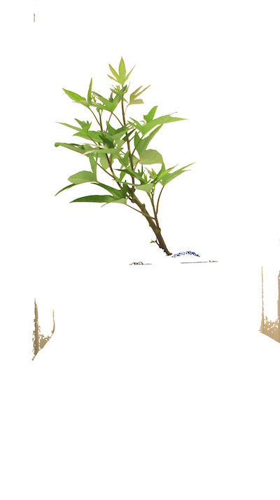
The image input by the user is read in.
### Main pipeline
def main():
    # Get options
    args = options()

    pcv.params.debug=args.debug #set debug mode
    pcv.params.debug_outdir=args.outdir #set output directory

    # Read image (readimage mode defaults to native but if image is RGBA then specify mode='rgb')
    img, path, filename = pcv.readimage(args.image, mode='rgb')
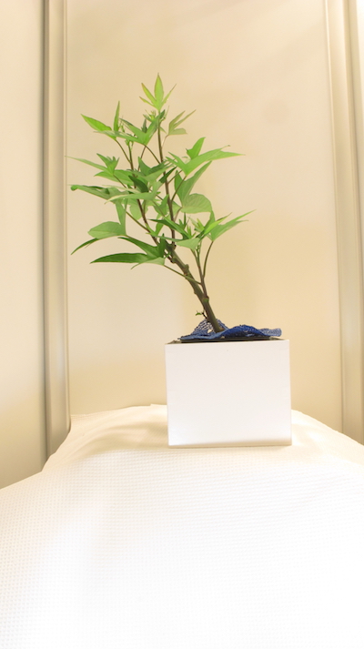
Figure 1. Original image. This particular image was captured by a digital camera, just to show that PlantCV works on images not captured on a high-throughput phenotyping system with idealized VIS image capture conditions.
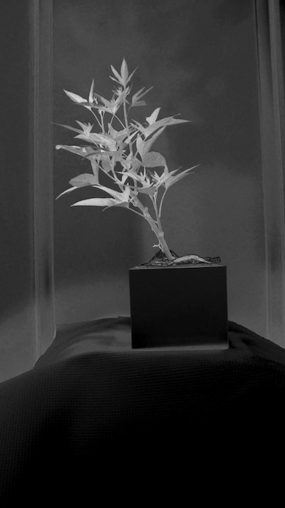
In some pipelines (especially ones captured with a high-throughput phenotyping systems, where background is predictable) we first threshold out background. In this particular pipeline we do some pre-masking of the background. The goal is to remove as much background as possible without losing any information from the plant. In order to perform a binary threshold on an image you need to select one of the color channels H,S,V,L,A,B,R,G,B. Here we convert the RGB image to HSV color space then extract the 's' or saturation channel, but any channel can be selected based on user need. If some of the plant is missed or not visible then thresholded channels may be combined (a later step).
    # Convert RGB to HSV and extract the saturation channel
    s = pcv.rgb2gray_hsv(img, 's')
Figure 2. Saturation channel from original RGB image converted to HSV color space.
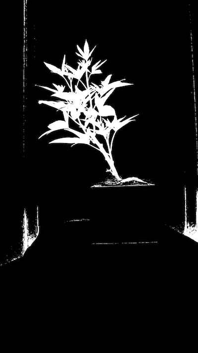
Next, the saturation channel is thresholded. The threshold can be on either light or dark objects in the image).
Tip: This step is often one that needs to be adjusted depending on the lighting and configurations of your camera system.
    # Threshold the saturation image
    s_thresh = pcv.threshold.binary(s, 85, 255, 'light')
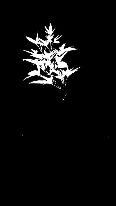
Figure 3. Thresholded saturation channel image (Figure 2). Remaining objects are in white.
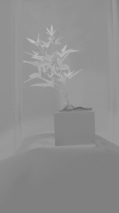
Again, depending on the lighting it will be possible to remove more/less background. A median blur can be used to remove noise.
Tip: Fill and median blur type steps should be used as sparingly as possible. Depending on the plant type (esp. grasses with thin leaves that often twist) you can lose plant material with a blur that is too harsh.
    # Median Blur
    s_mblur = pcv.median_blur(s_thresh, 5)
    s_cnt = pcv.median_blur(s_thresh, 5)
Figure 4. Thresholded saturation channel image with median blur.

Here is where the pipeline branches. The original image is converted from an RGB image to LAB color space and we extract blue-yellow channel. This image is again thresholded and there is an optional fill step that wasn't needed in this pipeline.
    # Convert RGB to LAB and extract the Blue channel
    b = pcv.rgb2gray_lab(img, 'b')

    # Threshold the blue image
    b_thresh = pcv.threshold.binary(b, 160, 255, 'light')
    b_cnt = pcv.threshold.binary(b, 160, 255, 'light')

    # Fill small objects
    #b_fill = pcv.fill(b_thresh, 10)
Figure 5. (Top) Blue-yellow channel from LAB color space from original image. (Bottom) Thresholded blue-yellow channel image.
Join the binary images from Figure 4 and Figure 5 with the logical or function.
    # Join the thresholded saturation and blue-yellow images
    bs = pcv.logical_or(s_mblur, b_cnt)
Figure 6. Joined binary images (Figure 4 and Figure 5).

Next, apply the binary image (Figure 6) as an image mask over the original image. The purpose of this mask is to exclude as much background with simple thresholding without leaving out plant material.
    # Apply Mask (for VIS images, mask_color=white)
    masked = pcv.apply_mask(img, bs, 'white')
Figure 7. Masked image with background removed.

Now we'll focus on capturing the plant in the masked image from Figure 7. The masked green-magenta and blue-yellow channels are extracted. Then the two channels are thresholded to capture different portions of the plant, and the three images are joined together. The small objects are filled. The resulting binary image is used to mask the masked image from Figure 7.
    # Convert RGB to LAB and extract the Green-Magenta and Blue-Yellow channels
    masked_a = pcv.rgb2gray_lab(masked, 'a')
    masked_b = pcv.rgb2gray_lab(masked, 'b')

    # Threshold the green-magenta and blue images
    maskeda_thresh = pcv.threshold.binary(masked_a, 115, 255, 'dark')
    maskeda_thresh1 = pcv.threshold.binary(masked_a, 135, 255, 'light')
    maskedb_thresh = pcv.threshold.binary(masked_b, 128, 255, 'light')

    # Join the thresholded saturation and blue-yellow images (OR)
    ab1 = pcv.logical_or(maskeda_thresh, maskedb_thresh)
    ab = pcv.logical_or(maskeda_thresh1, ab1)

    # Fill small objects
    ab_fill = pcv.fill(ab, 200)

    # Apply mask (for VIS images, mask_color=white)
    masked2 = pcv.apply_mask(masked, ab_fill, 'white')
The sample image used had very green leaves, but often (especially with stress treatments) there are yellowing leaves, redish leaves, or regions of necrosis. The different thresholding channels capture different regions of the plant, then are combined into a mask for the image that was previously masked (Figure 7).
Figure 8. RGB to LAB conversion. (Top) The green-magenta "a" channel image. (Bottom) The blue-yellow "b" channel image.

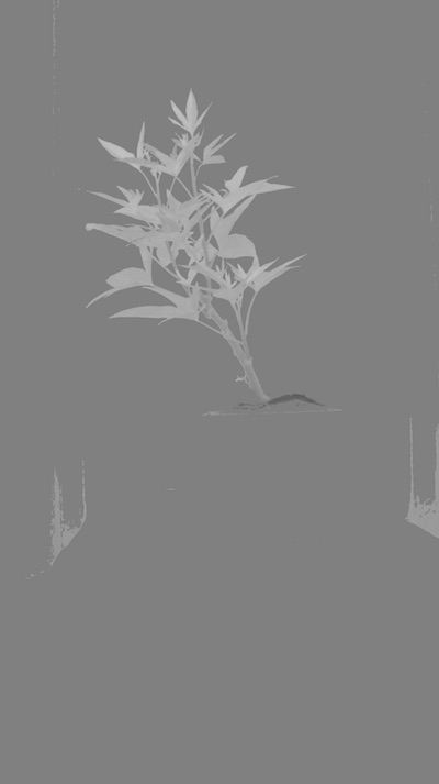
Figure 9. Thresholded LAB channel images. (Top) "dark" threshold 115. (Middle) "light" threshold 135. (Bottom) "light" threshold 128.

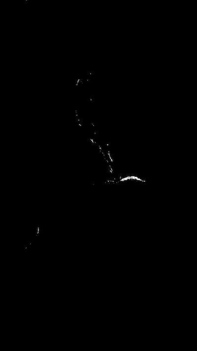

Figure 9. Combined thresholded images.


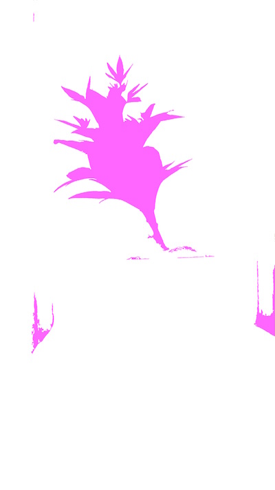
Figure 10. Fill in small objects. (Top) Image with objects < 200 px filled. (Bottom) Masked image.

Now we need to identify the objects (called contours in OpenCV) within the image.
    # Identify objects
    id_objects, obj_hierarchy = pcv.find_objects(masked2, ab_fill)
Figure 11. Here the objects (purple) are identified from the image from Figure 10. Even the spaces within an object are colored, but will have different hierarchy values.
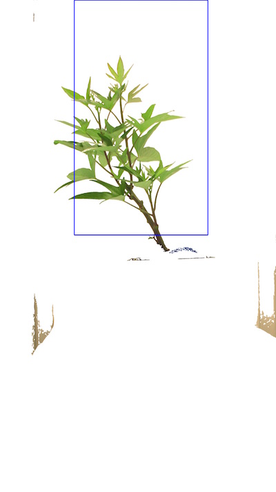
Next a rectangular region of interest is defined (this can be made on the fly).
    # Define ROI
    roi1, roi_hierarchy= pcv.roi.rectangle(img=masked2, x=100, y=100, h=200, w=200)
Figure 12. Region of interest drawn onto image.
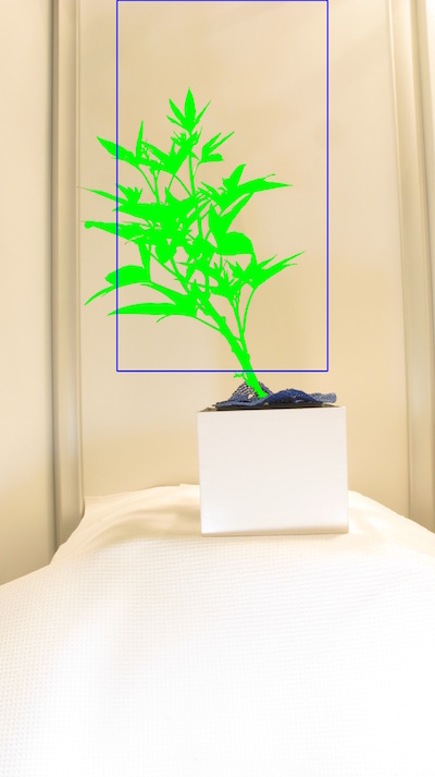
Once the region of interest is defined you can decide to keep everything overlapping with the region of interest) or cut the objects to the shape of the region of interest.
    # Decide which objects to keep
    roi_objects, hierarchy3, kept_mask, obj_area = pcv.roi_objects(img, 'partial', roi1, roi_hierarchy, id_objects, obj_hierarchy)
Figure 13. Kept objects (green) drawn onto image.
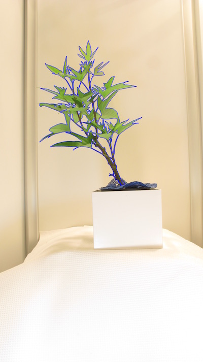
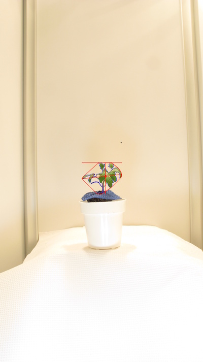
The isolated objects now should all be plant material. There can be more than one object that makes up a plant since sometimes leaves twist making them appear in images as separate objects. Therefore, in order for shape analysis to perform properly the plant objects need to be combined into one object using the combine objects function.
    # Object combine kept objects
    obj, mask = pcv.object_composition(img, roi_objects, hierarchy3)
Figure 14. Outline (blue) of combined objects on the image.
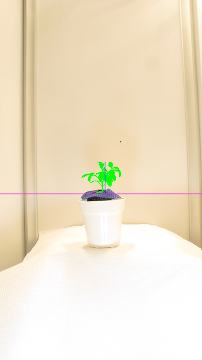
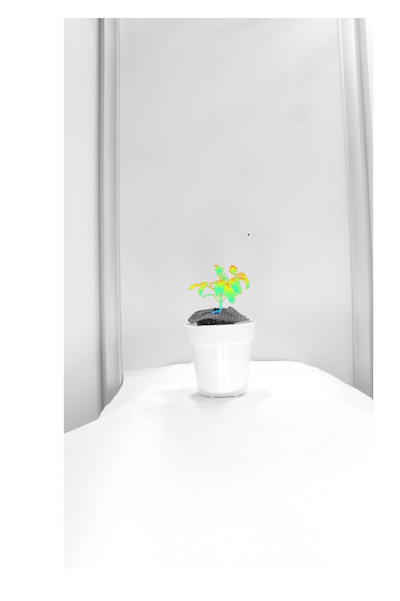
The next step is to analyze the plant object for traits such as horizontal height, shape, or color.
############### Analysis ################
outfile=False
if args.writeimg==True:
outfile=args.outdir+"/"+filename
# Find shape properties, output shape image (optional)
shape_header, shape_data, shape_imgs = pcv.analyze_object(img, obj, mask)
# Shape properties relative to user boundary line (optional)
boundary_header, boundary_data, boundary_img1 = pcv.analyze_bound_horizontal(img, obj, mask, 1680)
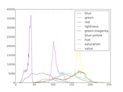
# Determine color properties: Histograms, Color Slices, output color analyzed histogram (optional)
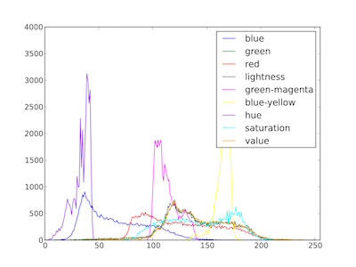
color_header, color_data, color_histogram = pcv.analyze_color(img, kept_mask, 256, 'all')
# Pseudocolor the grayscale image
pseudocolored_img = pcv.pseudocolor(gray_img=s, mask=kept_mask, cmap='jet')
# Write shape and color data to results file
pcv.print_results(filename=args.result)
if __name__ == '__main__':
main()
Figure 15. Shape analysis output image.
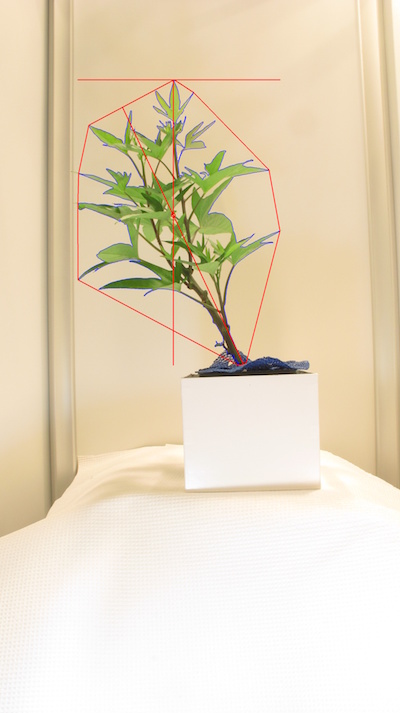
Figure 16. Boundary line output image.
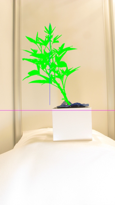
Figure 17. Pseudocolored image (based on value channel).
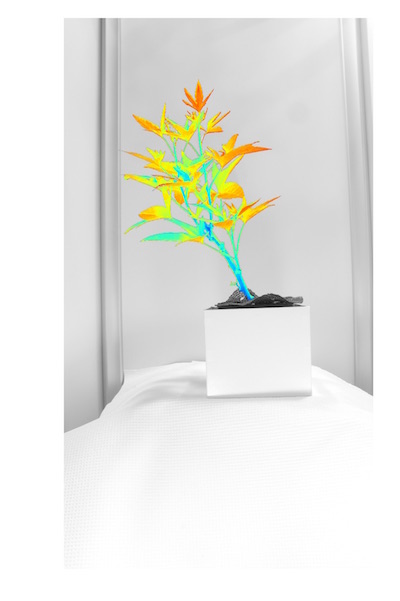
Figure 18. Histogram of color values for each plant pixel.
Additional examples
To demonstrate the importance of camera settings on pipeline construction here are different species of plants captured with the same imaging setup (digital camera) and processed with the same imaging pipeline as above (no settings changed).
Figure 19. Output images from Cassava trait analysis. (From top to bottom) Original image, shape output image, boundary line output image, pseudocolored image (based on value channel), histogram of color values for each plant pixel.
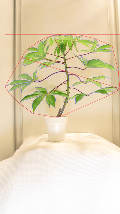
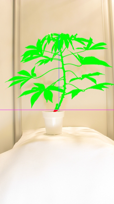
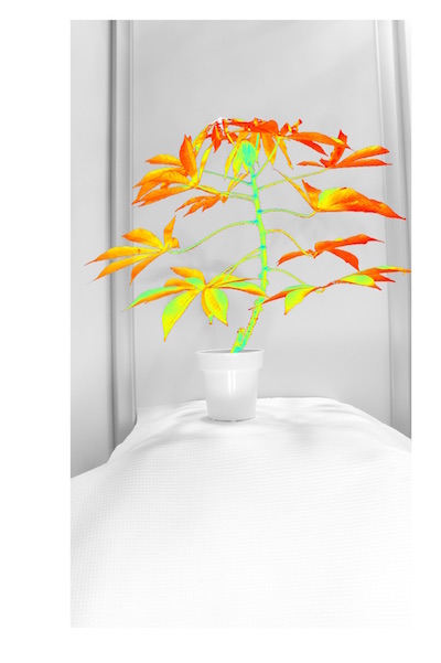
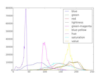
Figure 20. Output images from Tomato trait analysis. (From top to bottom) Original image, shape output image, boundary line output image, pseudocolored image (based on value channel), histogram of color values for each plant pixel.
To deploy a pipeline over a full image set please see tutorial on pipeline parallelization.
VIS Script
In the terminal:
./pipelinename.py -i testimg.png -o ./output-images -r results.txt -w -D 'print'
- Always test pipelines (preferably with -D flag set to 'print') before running over a full image set
Python script:
# !/usr/bin/python
import sys, traceback
import cv2
import numpy as np
import argparse
import string
from plantcv import plantcv as pcv


### Parse command-line arguments
def options():
    parser = argparse.ArgumentParser(description="Imaging processing with opencv")
    parser.add_argument("-i", "--image", help="Input image file.", required=True)
    parser.add_argument("-o", "--outdir", help="Output directory for image files.", required=False)
    parser.add_argument("-r", "--result", help="result file.", required=False)
    parser.add_argument("-w", "--writeimg", help="write out images.", default=False, action="store_true")
    parser.add_argument("-D", "--debug",
                        help="can be set to 'print' or None (or 'plot' if in jupyter) prints intermediate images.",
                        default=None)
    args = parser.parse_args()
    return args

#### Start of the Main/Customizable portion of the pipeline.

### Main pipeline
def main():
    # Get options
    args = options()

    pcv.params.debug = args.debug  # set debug mode
    pcv.params.debug_outdir = args.outdir  # set output directory

    # Read image
    img, path, filename = pcv.readimage(args.image)

    # Convert RGB to HSV and extract the saturation channel
    s = pcv.rgb2gray_hsv(img, 's')

    # Threshold the saturation image
    s_thresh = pcv.threshold.binary(s, 85, 255, 'light')

    # Median Blur
    s_mblur = pcv.median_blur(s_thresh, 5)
    s_cnt = pcv.median_blur(s_thresh, 5)

    # Convert RGB to LAB and extract the Blue channel
    b = pcv.rgb2gray_lab(img, 'b')

    # Threshold the blue image
    b_thresh = pcv.threshold.binary(b, 160, 255, 'light')
    b_cnt = pcv.threshold.binary(b, 160, 255, 'light')

    # Fill small objects
    # b_fill = pcv.fill(b_thresh, 10)

    # Join the thresholded saturation and blue-yellow images
    bs = pcv.logical_or(s_mblur, b_cnt)

    # Apply Mask (for VIS images, mask_color=white)
    masked = pcv.apply_mask(img, bs, 'white')

    # Convert RGB to LAB and extract the Green-Magenta and Blue-Yellow channels
    masked_a = pcv.rgb2gray_lab(masked, 'a')
    masked_b = pcv.rgb2gray_lab(masked, 'b')

    # Threshold the green-magenta and blue images
    maskeda_thresh = pcv.threshold.binary(masked_a, 115, 255, 'dark')
    maskeda_thresh1 = pcv.threshold.binary(masked_a, 135, 255, 'light')
    maskedb_thresh = pcv.threshold.binary(masked_b, 128, 255, 'light')

    # Join the thresholded saturation and blue-yellow images (OR)
    ab1 = pcv.logical_or(maskeda_thresh, maskedb_thresh)
    ab = pcv.logical_or(maskeda_thresh1, ab1)

    # Fill small objects
    ab_fill = pcv.fill(ab, 200)

    # Apply mask (for VIS images, mask_color=white)
    masked2 = pcv.apply_mask(masked, ab_fill, 'white')

    # Identify objects
    id_objects, obj_hierarchy = pcv.find_objects(masked2, ab_fill)

    # Define ROI
    roi1, roi_hierarchy= pcv.roi.rectangle(x=100, y=100, h=200, w=200, img=masked2)

    # Decide which objects to keep
    roi_objects, hierarchy3, kept_mask, obj_area = pcv.roi_objects(img, 'partial', roi1, roi_hierarchy, id_objects, obj_hierarchy)

    # Object combine kept objects
    obj, mask = pcv.object_composition(img, roi_objects, hierarchy3)

    ############### Analysis ################

    outfile=False
    if args.writeimg == True:
        outfile = args.outdir + "/" + filename

    # Find shape properties, output shape image (optional)
    shape_header, shape_data, shape_imgs = pcv.analyze_object(img, obj, mask)

    # Shape properties relative to user boundary line (optional)
    boundary_header, boundary_data, boundary_img1 = pcv.analyze_bound_horizontal(img, obj, mask, 1680)

    # Determine color properties: Histograms, Color Slices, output color analyzed histogram (optional)
    color_header, color_data, color_histogram = pcv.analyze_color(img, kept_mask, 256, 'all')

    # Pseudocolor the grayscale image
    pseudocolored_img = pcv.pseudocolor(gray_img=s, mask=kept_mask, cmap='jet')

    # Write shape and color data to results file
    pcv.print_results(filename=args.result)

if __name__ == '__main__':
    main()